Question 1. Think about an ongoing study in your lab (or a paper you
have read in a different class), and decide on a pattern that you might
expect in your experiment if a specific hypothesis were true.
I am in Dr. Mark Henderson’s lab studying catch per unit effort
(CPUE; fish/hr) of Atlantic Salmon in Lake Champlain using boat
electrofishing. We have generated CPUE of Atlantic Salmon catch rates
for a sampling protocol for fish collection for acoustic telemetry
studies. Understanding the optimal sampling time is beneficial for us
because we want to be most efficient while collecting fish in the field.
We are interested in how the water temperature of Lake Champlain effects
the CPUE of Atlantic Salmon. We hypothesize that as the water
temperature increases, the CPUE of Atlantic Salmon will decrease because
the Atlantic Salmon will be in deeper water and out of the electrical
field where we are shocking (<15 ft.). The Atlantic Salmon are
cold-water fish and want to live in the cooler and deeper waters when
the surface temperature is higher.
Question 2. To start simply, assume that the data in each of your
treatment groups follow a normal distribution. Specify the sample sizes,
means, and variances for each group that would be reasonable if your
hypothesis were true. You may need to consult some previous literature
and/or an expert in the field to come up with these numbers.
I am using mock electrofishing data collected from sampling Atlantic
Salmon with boat electrofishing in the Fall in Lake Champlain.
Question 3. Using the methods we have covered in class, write code
to create a random data set that has these attributes. Organize these
data into a data frame with the appropriate structure.
library(ggplot2)
library(dplyr)
##
## Attaching package: 'dplyr'
## The following objects are masked from 'package:stats':
##
##     filter, lag
## The following objects are masked from 'package:base':
##
##     intersect, setdiff, setequal, union
# Create the dataframe
?rnorm()

low <- data.frame(
  temp_group = "Low (2-4.9°C)",
  CPUE = rnorm(n = 20, mean = 18, sd = 1.2),
  temperature = runif(20, 2, 4.9))

print(low)
##       temp_group     CPUE temperature
## 1  Low (2-4.9°C) 18.49176    2.102723
## 2  Low (2-4.9°C) 16.90927    2.894233
## 3  Low (2-4.9°C) 18.16403    4.739052
## 4  Low (2-4.9°C) 17.21519    2.967240
## 5  Low (2-4.9°C) 15.64008    2.468065
## 6  Low (2-4.9°C) 19.81239    3.048556
## 7  Low (2-4.9°C) 16.62832    2.086770
## 8  Low (2-4.9°C) 18.96501    3.714125
## 9  Low (2-4.9°C) 18.81509    3.031670
## 10 Low (2-4.9°C) 18.21638    2.334705
## 11 Low (2-4.9°C) 17.14709    2.430502
## 12 Low (2-4.9°C) 18.46636    2.987518
## 13 Low (2-4.9°C) 17.64002    2.566809
## 14 Low (2-4.9°C) 18.51549    3.238843
## 15 Low (2-4.9°C) 17.73579    3.770052
## 16 Low (2-4.9°C) 15.81257    3.057632
## 17 Low (2-4.9°C) 17.99032    3.237038
## 18 Low (2-4.9°C) 19.79405    3.870421
## 19 Low (2-4.9°C) 19.79749    2.152623
## 20 Low (2-4.9°C) 19.94003    4.012127
medium <- data.frame(
  temp_group = "Medium (5-7.9°C)",
  CPUE = rnorm(n = 20, mean = 12, sd = 1.5),
  temperature = runif(20, 5, 7.9))

print(medium)
##          temp_group      CPUE temperature
## 1  Medium (5-7.9°C) 11.938600    6.107339
## 2  Medium (5-7.9°C) 11.453766    7.538831
## 3  Medium (5-7.9°C)  9.602795    6.933937
## 4  Medium (5-7.9°C) 13.244273    5.141880
## 5  Medium (5-7.9°C) 11.903236    6.946314
## 6  Medium (5-7.9°C) 11.176925    6.686907
## 7  Medium (5-7.9°C) 11.344432    6.377967
## 8  Medium (5-7.9°C) 12.729125    5.141475
## 9  Medium (5-7.9°C) 11.010088    7.094247
## 10 Medium (5-7.9°C) 11.188693    6.344357
## 11 Medium (5-7.9°C) 11.453883    6.154492
## 12 Medium (5-7.9°C) 12.307934    7.094248
## 13 Medium (5-7.9°C) 10.828742    6.411708
## 14 Medium (5-7.9°C) 14.282856    5.688156
## 15 Medium (5-7.9°C) 11.407783    7.808581
## 16 Medium (5-7.9°C) 11.790666    6.732025
## 17 Medium (5-7.9°C) 12.597948    6.922835
## 18 Medium (5-7.9°C)  9.784362    6.011354
## 19 Medium (5-7.9°C) 10.590386    6.980192
## 20 Medium (5-7.9°C) 13.264881    6.968713
high <- data.frame(
  temp_group = "High (8-10.9°C)",
  CPUE = rnorm(n = 20, mean = 8, sd = 2),
  temperature = runif(20, 8, 10.9))

print(high)
##         temp_group      CPUE temperature
## 1  High (8-10.9°C)  6.294073    9.122742
## 2  High (8-10.9°C)  6.547032   10.638677
## 3  High (8-10.9°C)  3.504796    9.478080
## 4  High (8-10.9°C)  9.188975    8.048538
## 5  High (8-10.9°C)  8.853694    8.157085
## 6  High (8-10.9°C) 11.329284    8.220140
## 7  High (8-10.9°C)  9.006154   10.741013
## 8  High (8-10.9°C)  8.780301   10.728099
## 9  High (8-10.9°C)  9.970275    9.185166
## 10 High (8-10.9°C)  8.921591    8.754799
## 11 High (8-10.9°C)  6.817733    8.791094
## 12 High (8-10.9°C)  8.975112    8.536939
## 13 High (8-10.9°C)  4.943874    9.236420
## 14 High (8-10.9°C)  9.806812   10.269482
## 15 High (8-10.9°C)  9.921124    9.503365
## 16 High (8-10.9°C)  6.091875    9.073177
## 17 High (8-10.9°C) 11.685133    9.413965
## 18 High (8-10.9°C)  5.684252    9.539796
## 19 High (8-10.9°C)  3.307066    8.223623
## 20 High (8-10.9°C)  7.914440    8.244499
# combine all of the the datasets together to make a big dataset with low, medium, and high datasets
data <- rbind(low, medium, high)

print(data)
##          temp_group      CPUE temperature
## 1     Low (2-4.9°C) 18.491758    2.102723
## 2     Low (2-4.9°C) 16.909266    2.894233
## 3     Low (2-4.9°C) 18.164032    4.739052
## 4     Low (2-4.9°C) 17.215192    2.967240
## 5     Low (2-4.9°C) 15.640075    2.468065
## 6     Low (2-4.9°C) 19.812391    3.048556
## 7     Low (2-4.9°C) 16.628318    2.086770
## 8     Low (2-4.9°C) 18.965010    3.714125
## 9     Low (2-4.9°C) 18.815086    3.031670
## 10    Low (2-4.9°C) 18.216381    2.334705
## 11    Low (2-4.9°C) 17.147087    2.430502
## 12    Low (2-4.9°C) 18.466359    2.987518
## 13    Low (2-4.9°C) 17.640024    2.566809
## 14    Low (2-4.9°C) 18.515487    3.238843
## 15    Low (2-4.9°C) 17.735790    3.770052
## 16    Low (2-4.9°C) 15.812570    3.057632
## 17    Low (2-4.9°C) 17.990315    3.237038
## 18    Low (2-4.9°C) 19.794053    3.870421
## 19    Low (2-4.9°C) 19.797495    2.152623
## 20    Low (2-4.9°C) 19.940035    4.012127
## 21 Medium (5-7.9°C) 11.938600    6.107339
## 22 Medium (5-7.9°C) 11.453766    7.538831
## 23 Medium (5-7.9°C)  9.602795    6.933937
## 24 Medium (5-7.9°C) 13.244273    5.141880
## 25 Medium (5-7.9°C) 11.903236    6.946314
## 26 Medium (5-7.9°C) 11.176925    6.686907
## 27 Medium (5-7.9°C) 11.344432    6.377967
## 28 Medium (5-7.9°C) 12.729125    5.141475
## 29 Medium (5-7.9°C) 11.010088    7.094247
## 30 Medium (5-7.9°C) 11.188693    6.344357
## 31 Medium (5-7.9°C) 11.453883    6.154492
## 32 Medium (5-7.9°C) 12.307934    7.094248
## 33 Medium (5-7.9°C) 10.828742    6.411708
## 34 Medium (5-7.9°C) 14.282856    5.688156
## 35 Medium (5-7.9°C) 11.407783    7.808581
## 36 Medium (5-7.9°C) 11.790666    6.732025
## 37 Medium (5-7.9°C) 12.597948    6.922835
## 38 Medium (5-7.9°C)  9.784362    6.011354
## 39 Medium (5-7.9°C) 10.590386    6.980192
## 40 Medium (5-7.9°C) 13.264881    6.968713
## 41  High (8-10.9°C)  6.294073    9.122742
## 42  High (8-10.9°C)  6.547032   10.638677
## 43  High (8-10.9°C)  3.504796    9.478080
## 44  High (8-10.9°C)  9.188975    8.048538
## 45  High (8-10.9°C)  8.853694    8.157085
## 46  High (8-10.9°C) 11.329284    8.220140
## 47  High (8-10.9°C)  9.006154   10.741013
## 48  High (8-10.9°C)  8.780301   10.728099
## 49  High (8-10.9°C)  9.970275    9.185166
## 50  High (8-10.9°C)  8.921591    8.754799
## 51  High (8-10.9°C)  6.817733    8.791094
## 52  High (8-10.9°C)  8.975112    8.536939
## 53  High (8-10.9°C)  4.943874    9.236420
## 54  High (8-10.9°C)  9.806812   10.269482
## 55  High (8-10.9°C)  9.921124    9.503365
## 56  High (8-10.9°C)  6.091875    9.073177
## 57  High (8-10.9°C) 11.685133    9.413965
## 58  High (8-10.9°C)  5.684252    9.539796
## 59  High (8-10.9°C)  3.307066    8.223623
## 60  High (8-10.9°C)  7.914440    8.244499
# Question 4. Now write code to analyze the data (probably as an ANOVA or regression analysis, but possibly as a logistic regression or contingency table analysis. Write code to generate a useful graph of the data.

# First, we can do a linear regression on the continuous variables
# Fit linear model
linear_regression <- lm(CPUE ~ temperature, data = data)

print(linear_regression)
##
## Call:
## lm(formula = CPUE ~ temperature, data = data)
##
## Coefficients:
## (Intercept)  temperature
##       22.13        -1.53
my_out <- c(slope=summary(linear_regression)$coefficients[2,1],
            p_value=summary(linear_regression)$coefficients[2,4],
            r_squared = summary(linear_regression)$r.squared)

print(summary(linear_regression))
##
## Call:
## lm(formula = CPUE ~ temperature, data = data)
##
## Residuals:
##     Min      1Q  Median      3Q     Max
## -6.2436 -1.3237 -0.3064  1.3252  3.9556
##
## Coefficients:
##             Estimate Std. Error t value Pr(>|t|)
## (Intercept)  22.1326     0.6993   31.65   <2e-16 ***
## temperature  -1.5300     0.1030  -14.86   <2e-16 ***
## ---
## Signif. codes:  0 '***' 0.001 '**' 0.01 '*' 0.05 '.' 0.1 ' ' 1
##
## Residual standard error: 2.098 on 58 degrees of freedom
## Multiple R-squared:  0.792,  Adjusted R-squared:  0.7884
## F-statistic: 220.8 on 1 and 58 DF,  p-value: < 2.2e-16
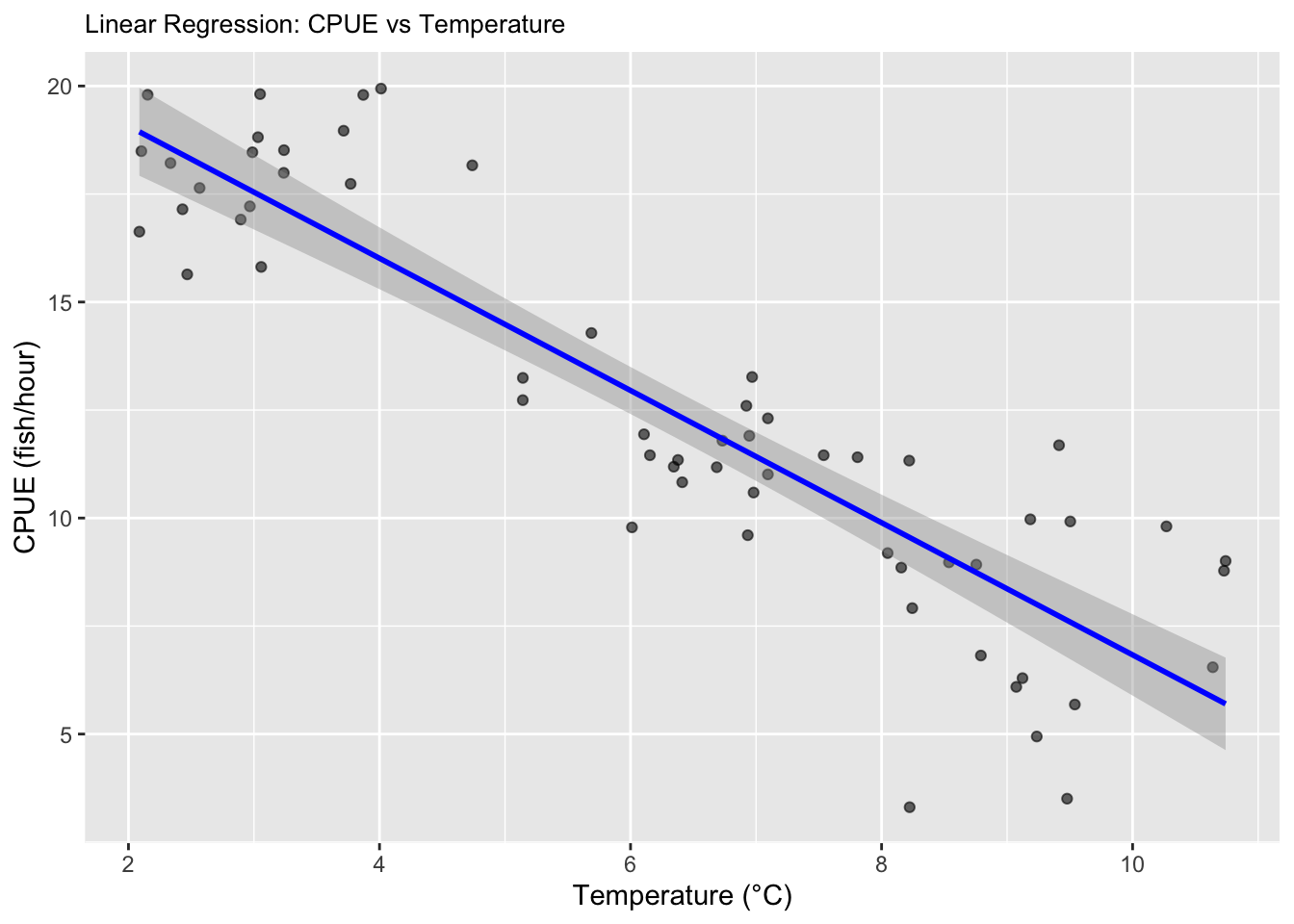
# Visualizations
# Create scatter plot with regression line
salmon_plot <- ggplot(data, aes(x = temperature, y = CPUE)) +
  geom_point(alpha = 0.6) +
  geom_smooth(method = "lm", color = "blue") +
  labs(
    title = "Linear Regression: CPUE vs Temperature",
    x = "Temperature (°C)",
    y = "CPUE (fish/hour)"
  ) + theme(plot.title = element_text(size = 10));salmon_plot
## `geom_smooth()` using formula = 'y ~ x'
print(salmon_plot)
## `geom_smooth()` using formula = 'y ~ x'

Question 5. Try running your analysis multiple times to get a
feeling for how variable the results are with the same parameters, but
different sets of random numbers.
I have rerun the code above so that the random numbers change each
time to see the differences!
Question 6. Now, using a series of for loops, adjust the parameters
of your data to explore how they might impact your results/analysis, and
store the results of your for loops into an object so you can view it.
For example, what happens if you were to start with a small sample size
and then re-run your analysis? Would you still get a significant result?
What if you were to increase that sample size by 5, or 10? How small can
your sample size be before you detect a significant pattern (p <
0.05)? How small can the differences between the groups be (the “effect
size”) for you to still detect a significant pattern?
# Set seed for reproducibility
set.seed(25)

# Change sample sizes, decreasing sample sizes
m <- c(2,3,4,5,6,7,8,9,10,15)
for (i in seq_along(m)){
  print(m[i])
  low <- data.frame(
    temp_group = "Low (2-4.9°C)",
    CPUE = rnorm(n = m[i], mean = 10, sd = 1.2),
    temperature = runif(m[i], 2, 4.9));low

  medium <- data.frame(
    temp_group = "Medium (5-7.9°C)",
    CPUE = rnorm(n = m[i], mean = 6, sd = 1.3),
    temperature = runif(m[i], 5, 7.9));medium

  high <- data.frame(
    temp_group = "High (8-10.9°C)",
    CPUE = rnorm(n = m[i], mean = 4, sd = 1.3),
    temperature = runif(m[i], 8, 10.9));high
  data <- rbind(low, medium, high)
  linear_regression <- lm(CPUE ~ temperature, data = data)

  my_out <- c(slope=summary(linear_regression)$coefficients[2,1],
              p_value=summary(linear_regression)$coefficients[2,4],
              r_squared = summary(linear_regression)$r.squared);my_out

  print(summary(linear_regression))

}
## [1] 2
##
## Call:
## lm(formula = CPUE ~ temperature, data = data)
##
## Residuals:
##          1          2          3          4          5          6
##  0.8469007  1.2145919 -0.5198041 -2.8316596  1.2904690 -0.0004979
##
## Coefficients:
##             Estimate Std. Error t value Pr(>|t|)
## (Intercept)  10.1884     1.8682   5.454  0.00549 **
## temperature  -0.5462     0.2664  -2.050  0.10969
## ---
## Signif. codes:  0 '***' 0.001 '**' 0.01 '*' 0.05 '.' 0.1 ' ' 1
##
## Residual standard error: 1.743 on 4 degrees of freedom
## Multiple R-squared:  0.5123, Adjusted R-squared:  0.3904
## F-statistic: 4.202 on 1 and 4 DF,  p-value: 0.1097
##
## [1] 3
##
## Call:
## lm(formula = CPUE ~ temperature, data = data)
##
## Residuals:
##     Min      1Q  Median      3Q     Max
## -1.2387 -0.5525 -0.4107  0.4796  1.7739
##
## Coefficients:
##             Estimate Std. Error t value Pr(>|t|)
## (Intercept)  10.0502     0.8776  11.452  8.7e-06 ***
## temperature  -0.6029     0.1268  -4.755  0.00207 **
## ---
## Signif. codes:  0 '***' 0.001 '**' 0.01 '*' 0.05 '.' 0.1 ' ' 1
##
## Residual standard error: 1.133 on 7 degrees of freedom
## Multiple R-squared:  0.7636, Adjusted R-squared:  0.7298
## F-statistic: 22.61 on 1 and 7 DF,  p-value: 0.002071
##
## [1] 4
##
## Call:
## lm(formula = CPUE ~ temperature, data = data)
##
## Residuals:
##     Min      1Q  Median      3Q     Max
## -2.0370 -0.2571  0.2918  0.6447  1.1882
##
## Coefficients:
##             Estimate Std. Error t value Pr(>|t|)
## (Intercept)  13.0428     0.7764  16.800 1.17e-08 ***
## temperature  -1.0128     0.1111  -9.115 3.69e-06 ***
## ---
## Signif. codes:  0 '***' 0.001 '**' 0.01 '*' 0.05 '.' 0.1 ' ' 1
##
## Residual standard error: 1.049 on 10 degrees of freedom
## Multiple R-squared:  0.8926, Adjusted R-squared:  0.8818
## F-statistic: 83.08 on 1 and 10 DF,  p-value: 3.691e-06
##
## [1] 5
##
## Call:
## lm(formula = CPUE ~ temperature, data = data)
##
## Residuals:
##     Min      1Q  Median      3Q     Max
## -2.7083 -0.6493 -0.1143  1.0652  2.3842
##
## Coefficients:
##             Estimate Std. Error t value Pr(>|t|)
## (Intercept)  12.2416     1.0519  11.638 3.02e-08 ***
## temperature  -0.9881     0.1549  -6.379 2.42e-05 ***
## ---
## Signif. codes:  0 '***' 0.001 '**' 0.01 '*' 0.05 '.' 0.1 ' ' 1
##
## Residual standard error: 1.577 on 13 degrees of freedom
## Multiple R-squared:  0.7579, Adjusted R-squared:  0.7393
## F-statistic:  40.7 on 1 and 13 DF,  p-value: 2.42e-05
##
## [1] 6
##
## Call:
## lm(formula = CPUE ~ temperature, data = data)
##
## Residuals:
##     Min      1Q  Median      3Q     Max
## -2.6086 -0.7090  0.2239  0.6371  2.1014
##
## Coefficients:
##             Estimate Std. Error t value Pr(>|t|)
## (Intercept)  12.9854     0.8334   15.58 4.32e-11 ***
## temperature  -1.0271     0.1200   -8.56 2.28e-07 ***
## ---
## Signif. codes:  0 '***' 0.001 '**' 0.01 '*' 0.05 '.' 0.1 ' ' 1
##
## Residual standard error: 1.279 on 16 degrees of freedom
## Multiple R-squared:  0.8208, Adjusted R-squared:  0.8096
## F-statistic: 73.28 on 1 and 16 DF,  p-value: 2.28e-07
##
## [1] 7
##
## Call:
## lm(formula = CPUE ~ temperature, data = data)
##
## Residuals:
##     Min      1Q  Median      3Q     Max
## -3.0736 -1.4616 -0.1995  1.5237  3.8252
##
## Coefficients:
##             Estimate Std. Error t value Pr(>|t|)
## (Intercept)  12.4245     1.1364  10.933 1.23e-09 ***
## temperature  -0.8355     0.1631  -5.124 6.03e-05 ***
## ---
## Signif. codes:  0 '***' 0.001 '**' 0.01 '*' 0.05 '.' 0.1 ' ' 1
##
## Residual standard error: 2.075 on 19 degrees of freedom
## Multiple R-squared:  0.5802, Adjusted R-squared:  0.5581
## F-statistic: 26.26 on 1 and 19 DF,  p-value: 6.03e-05
##
## [1] 8
##
## Call:
## lm(formula = CPUE ~ temperature, data = data)
##
## Residuals:
##     Min      1Q  Median      3Q     Max
## -3.0045 -1.3996  0.1014  1.0751  2.1870
##
## Coefficients:
##             Estimate Std. Error t value Pr(>|t|)
## (Intercept)  12.8518     0.8163  15.743 1.85e-13 ***
## temperature  -0.9032     0.1143  -7.906 7.18e-08 ***
## ---
## Signif. codes:  0 '***' 0.001 '**' 0.01 '*' 0.05 '.' 0.1 ' ' 1
##
## Residual standard error: 1.586 on 22 degrees of freedom
## Multiple R-squared:  0.7396, Adjusted R-squared:  0.7278
## F-statistic:  62.5 on 1 and 22 DF,  p-value: 7.184e-08
##
## [1] 9
##
## Call:
## lm(formula = CPUE ~ temperature, data = data)
##
## Residuals:
##     Min      1Q  Median      3Q     Max
## -2.6962 -1.1016 -0.4546  0.9743  4.2637
##
## Coefficients:
##             Estimate Std. Error t value Pr(>|t|)
## (Intercept)  13.2322     0.8820  15.003 5.22e-14 ***
## temperature  -0.9206     0.1278  -7.202 1.51e-07 ***
## ---
## Signif. codes:  0 '***' 0.001 '**' 0.01 '*' 0.05 '.' 0.1 ' ' 1
##
## Residual standard error: 1.718 on 25 degrees of freedom
## Multiple R-squared:  0.6748, Adjusted R-squared:  0.6617
## F-statistic: 51.87 on 1 and 25 DF,  p-value: 1.511e-07
##
## [1] 10
##
## Call:
## lm(formula = CPUE ~ temperature, data = data)
##
## Residuals:
##      Min       1Q   Median       3Q      Max
## -2.53824 -0.83461  0.08895  0.78612  2.39261
##
## Coefficients:
##             Estimate Std. Error t value Pr(>|t|)
## (Intercept) 11.93585    0.65594  18.197  < 2e-16 ***
## temperature -0.80439    0.09302  -8.648 2.15e-09 ***
## ---
## Signif. codes:  0 '***' 0.001 '**' 0.01 '*' 0.05 '.' 0.1 ' ' 1
##
## Residual standard error: 1.4 on 28 degrees of freedom
## Multiple R-squared:  0.7276, Adjusted R-squared:  0.7178
## F-statistic: 74.78 on 1 and 28 DF,  p-value: 2.147e-09
##
## [1] 15
##
## Call:
## lm(formula = CPUE ~ temperature, data = data)
##
## Residuals:
##     Min      1Q  Median      3Q     Max
## -3.0690 -1.2985 -0.1933  1.3796  2.8533
##
## Coefficients:
##             Estimate Std. Error t value Pr(>|t|)
## (Intercept) 12.22348    0.65825  18.570  < 2e-16 ***
## temperature -0.85161    0.09315  -9.142 1.22e-11 ***
## ---
## Signif. codes:  0 '***' 0.001 '**' 0.01 '*' 0.05 '.' 0.1 ' ' 1
##
## Residual standard error: 1.61 on 43 degrees of freedom
## Multiple R-squared:  0.6603, Adjusted R-squared:  0.6524
## F-statistic: 83.58 on 1 and 43 DF,  p-value: 1.222e-11
I wanted to test if changing the sample sizes would impact the
p-value and r-squared of the regression. I found a significant
difference (p < 0.05) with 20 samples, so I wanted to see how if I
decreased the sample size that at what sample size I would not see a
significant difference. Therefore, I created a for loop and included
various sample sizes and found that at 2 sample sizes, I did not see a
significant difference. So, a sample size of 3 would be the effective
sample size (this is the answer for Question 7).
# Change the means for each temp group for sample size of 20
mean_low <- c(5, 6, 7, 8, 9, 10, 11)
for (i in seq_along(mean_low)){
  print(mean_low[i])
  low <- data.frame(
    temp_group = "Low (2-4.9°C)",
    CPUE = rnorm(n = 20, mean = mean_low[i], sd = 1.2),
    temperature = runif(20, 2, 4.9));low

  medium <- data.frame(
    temp_group = "Medium (5-7.9°C)",
    CPUE = rnorm(n = m[i], mean = 6, sd = 1.3),
    temperature = runif(m[i], 5, 7.9));medium

  high <- data.frame(
    temp_group = "High (8-10.9°C)",
    CPUE = rnorm(n = m[i], mean = 4, sd = 1.3),
    temperature = runif(m[i], 8, 10.9));high
  data <- rbind(low, medium, high)
  linear_regression <- lm(CPUE ~ temperature, data = data)

  my_out <- c(slope=summary(linear_regression)$coefficients[2,1],
              p_value=summary(linear_regression)$coefficients[2,4],
              r_squared = summary(linear_regression)$r.squared);my_out

  print(summary(linear_regression))

}
## [1] 5
##
## Call:
## lm(formula = CPUE ~ temperature, data = data)
##
## Residuals:
##     Min      1Q  Median      3Q     Max
## -2.9305 -0.6873  0.0905  1.0142  2.4402
##
## Coefficients:
##             Estimate Std. Error t value Pr(>|t|)
## (Intercept)   3.9025     0.7308   5.340 2.32e-05 ***
## temperature   0.2206     0.1460   1.511    0.145
## ---
## Signif. codes:  0 '***' 0.001 '**' 0.01 '*' 0.05 '.' 0.1 ' ' 1
##
## Residual standard error: 1.523 on 22 degrees of freedom
## Multiple R-squared:  0.09404,    Adjusted R-squared:  0.05286
## F-statistic: 2.284 on 1 and 22 DF,  p-value: 0.145
##
## [1] 6
##
## Call:
## lm(formula = CPUE ~ temperature, data = data)
##
## Residuals:
##     Min      1Q  Median      3Q     Max
## -2.1438 -0.7516 -0.1246  0.6296  2.1268
##
## Coefficients:
##             Estimate Std. Error t value Pr(>|t|)
## (Intercept)   7.1362     0.5323  13.407 1.22e-12 ***
## temperature  -0.4297     0.1146  -3.749  0.00099 ***
## ---
## Signif. codes:  0 '***' 0.001 '**' 0.01 '*' 0.05 '.' 0.1 ' ' 1
##
## Residual standard error: 1.109 on 24 degrees of freedom
## Multiple R-squared:  0.3694, Adjusted R-squared:  0.3431
## F-statistic: 14.06 on 1 and 24 DF,  p-value: 0.0009903
##
## [1] 7
##
## Call:
## lm(formula = CPUE ~ temperature, data = data)
##
## Residuals:
##     Min      1Q  Median      3Q     Max
## -2.0482 -0.4912  0.1494  0.4754  2.1363
##
## Coefficients:
##             Estimate Std. Error t value Pr(>|t|)
## (Intercept)  8.95120    0.43078   20.78  < 2e-16 ***
## temperature -0.46463    0.07915   -5.87 3.44e-06 ***
## ---
## Signif. codes:  0 '***' 0.001 '**' 0.01 '*' 0.05 '.' 0.1 ' ' 1
##
## Residual standard error: 1.088 on 26 degrees of freedom
## Multiple R-squared:  0.5699, Adjusted R-squared:  0.5534
## F-statistic: 34.46 on 1 and 26 DF,  p-value: 3.445e-06
##
## [1] 8
##
## Call:
## lm(formula = CPUE ~ temperature, data = data)
##
## Residuals:
##      Min       1Q   Median       3Q      Max
## -2.90192 -1.09600  0.07461  1.03858  2.27477
##
## Coefficients:
##             Estimate Std. Error t value Pr(>|t|)
## (Intercept)  10.3087     0.5958  17.302  < 2e-16 ***
## temperature  -0.7039     0.1070  -6.578 3.93e-07 ***
## ---
## Signif. codes:  0 '***' 0.001 '**' 0.01 '*' 0.05 '.' 0.1 ' ' 1
##
## Residual standard error: 1.407 on 28 degrees of freedom
## Multiple R-squared:  0.6071, Adjusted R-squared:  0.5931
## F-statistic: 43.27 on 1 and 28 DF,  p-value: 3.925e-07
##
## [1] 9
##
## Call:
## lm(formula = CPUE ~ temperature, data = data)
##
## Residuals:
##     Min      1Q  Median      3Q     Max
## -3.7049 -1.1223  0.3037  1.1845  2.8334
##
## Coefficients:
##             Estimate Std. Error t value Pr(>|t|)
## (Intercept)  12.4398     0.6118   20.33  < 2e-16 ***
## temperature  -0.8269     0.1034   -8.00 6.27e-09 ***
## ---
## Signif. codes:  0 '***' 0.001 '**' 0.01 '*' 0.05 '.' 0.1 ' ' 1
##
## Residual standard error: 1.502 on 30 degrees of freedom
## Multiple R-squared:  0.6808, Adjusted R-squared:  0.6702
## F-statistic: 63.99 on 1 and 30 DF,  p-value: 6.272e-09
##
## [1] 10
##
## Call:
## lm(formula = CPUE ~ temperature, data = data)
##
## Residuals:
##      Min       1Q   Median       3Q      Max
## -2.33207 -1.01424 -0.04888  1.00854  2.40947
##
## Coefficients:
##             Estimate Std. Error t value Pr(>|t|)
## (Intercept)  13.0303     0.5104   25.53  < 2e-16 ***
## temperature  -0.9005     0.0858  -10.49 6.85e-12 ***
## ---
## Signif. codes:  0 '***' 0.001 '**' 0.01 '*' 0.05 '.' 0.1 ' ' 1
##
## Residual standard error: 1.321 on 32 degrees of freedom
## Multiple R-squared:  0.7749, Adjusted R-squared:  0.7679
## F-statistic: 110.2 on 1 and 32 DF,  p-value: 6.854e-12
##
## [1] 11
##
## Call:
## lm(formula = CPUE ~ temperature, data = data)
##
## Residuals:
##     Min      1Q  Median      3Q     Max
## -3.6385 -0.7122  0.1809  0.7864  3.2821
##
## Coefficients:
##             Estimate Std. Error t value Pr(>|t|)
## (Intercept) 13.85992    0.61717  22.457  < 2e-16 ***
## temperature -0.97028    0.09893  -9.807 1.91e-11 ***
## ---
## Signif. codes:  0 '***' 0.001 '**' 0.01 '*' 0.05 '.' 0.1 ' ' 1
##
## Residual standard error: 1.533 on 34 degrees of freedom
## Multiple R-squared:  0.7388, Adjusted R-squared:  0.7312
## F-statistic: 96.19 on 1 and 34 DF,  p-value: 1.915e-11
The lower the mean is for the low temperature group, the less the p
value gets from the regression analysis. This does mot really have any
significant management implications because you really can not alter the
means (the data is the data that you collect) however, for practicing
the for loop, it was helpful to do.
Question 7. Alternatively, for the effect sizes you originally
hypothesized, what is the minimum sample size you would need in order to
detect a statistically significant effect? Again, run the model a few
times with the same parameter set to get a feeling for the effect of
random variation in the data.
Question 8. Write up your results in a markdown file, organized with
headers and different code chunks to show your analysis. Be explicit in
your explanation and justification for sample sizes, means, and
variances.
Complete